39 how to label bars in excel

How to Create Progress Bars in Excel With Conditional Formatting 11.03.2011 · Progress Bars in Excel 2010 “Bar-type” conditional formatting has been around since Excel 2007. But Excel 2007 would only make bars with a gradient – the bar would get paler and paler towards the end, so even at 100% it wouldn’t really look like 100%. Excel 2010 addresses this by adding Solid Fill bars that maintain one color all ... Data Labels above bar chart - Excel Help Forum You can link the data labels to other cells to display anything you want. Free addin to link labels to cells Attached Files 1142048b.xlsx‎ (21.0 KB, 18 views) Download Register To Reply Similar Threads

› office-addins-blog › 2018/10/10Find, label and highlight a certain data point in Excel ... Oct 10, 2018 · Select the Data Labels box and choose where to position the label. By default, Excel shows one numeric value for the label, y value in our case. To display both x and y values, right-click the label, click Format Data Labels…, select the X Value and Y value boxes, and set the Separator of your choosing: Label the data point by name

How to label bars in excel

Add a label or text box to a worksheet - support.microsoft.com A label identifies the purpose of a cell or text box, displays brief instructions, or provides a title or caption. A label can also display a descriptive picture. Use a label for flexible placement of instructions, to emphasize text, and when merged cells or a … How to Add Total Data Labels to the Excel Stacked Bar Chart Step 5: Right click your new data labels and format them so that their label position is "Above"; also make the labels bold and increase the font size. Step 6: Right click the line, select "Format Data Series"; in the Line Color menu, select "No line" Step 7: Delete the "Total" data series label within the legend HOW TO CREATE A BAR CHART WITH LABELS ABOVE BAR IN EXCEL - simplexCT In the chart, right-click the Series "Dummy" Data Labels and then, on the short-cut menu, click Format Data Labels. 15. In the Format Data Labels pane, under Label Options selected, set the Label Position to Inside End. 16. Next, while the labels are still selected, click on Text Options, and then click on the Textbox icon. 17.

How to label bars in excel. Swimmer Plots in Excel - Peltier Tech 08.09.2014 · A reader of the Peltier Tech Blog asked me about Swimmer Plots. The first chart below is taken from “Swimmer Plot: Tell a Graphical Story of Your Time to Response Data Using PROC SGPLOT (pdf)“, by Stacey Phillips, via Swimmer Plot by Sanjay Matange on the Graphically Speaking SAS blog. The swimmer chart below is an attempt to show the … › Labels › cat_CL142725Labels | Product, Shipping & Address Labels | Staples® Label products or ship packages with this 300-count pack of Avery Easy Peel print-to-the-edge 2 x 2-inch white square labels. Ideal for product branding, party favors and decorations, crafts, addressing and labeling food containers › 2018/09/12 › add-line-excel-graphHow to add a line in Excel graph (average line, benchmark ... Sep 12, 2018 · Select the last data point on the line and add a data label to it as discussed in the previous tip. Click on the label to select it, then click inside the label box, delete the existing value and type your text: Hover over the label box until your mouse pointer changes to a four-sided arrow, and then drag the label slightly above the line: How to Create Bar of Pie Chart in Excel? Step-by-Step In other words, we want the larger portions to remain in the pie and move the smaller portions to the stacked bar. For this follow the steps outlined below: Right-click on any slice of the pie chart. Select ' Format Data Series ' from the context menu that appears. This will open the 'Format Data Series ' sidebar to the right of the Excel window.

Error bars in Excel: standard and custom - Ablebits I am developing a grid chart for STAKEHOLDER MAPPING. I want the names of the stakeholders to show on the chart as labels but when two or more stakeholders have the same score their names are not listed separately, the are combined and therefore cannot be read. How to Label Axes in Excel: 6 Steps (with Pictures) - wikiHow Steps Download Article. 1. Open your Excel document. Double-click an Excel document that contains a graph. If you haven't yet created the document, open Excel and click Blank workbook, then create your graph before continuing. 2. Select the graph. Click your graph to select it. 3. Data labels on Up/Down Bars? | MrExcel Message Board You would need to add another element to the chart that does support labels. Here are two approaches: Method 1. Don't use up-down bars at all but instead use stacked columns to add the floating bar. Here is the data I used for my example. The yellow and gray columns are your original data. Histogram with Actual Bin Labels Between Bars - Peltier Tech Select the added series (select the visible series and press the up arrow key, or use one of the chart element picker dropdowns on the ribbon or right click menu), then click the menu key between the Alt and Ctrl keys to the right of the Space bar. This pops up the right click menu. Select Change Series Chart Type, and select one of the Line types.

Text Labels on a Horizontal Bar Chart in Excel - Peltier Tech On the Excel 2007 Chart Tools > Layout tab, click Axes, then Secondary Horizontal Axis, then Show Left to Right Axis. Now the chart has four axes. We want the Rating labels at the bottom of the chart, and we'll place the numerical axis at the top before we hide it. In turn, select the left and right vertical axes. How to Create Barcodes in Excel (Easy Step-by-Step) Below are the steps to install the Barcode font on your system so it's also available in Excel: Double-click the ZIP folder of the Code 39 font (that you downloaded from the above link) Double-click the .TTF file (when you open a file, you can see the preview of the font) Click on Install. This will install the font on your system support.microsoft.com › en-us › officeAdd a label or text box to a worksheet - support.microsoft.com Add a label (Form control) Click Developer, click Insert, and then click Label . Click the worksheet location where you want the upper-left corner of the label to appear. To specify the control properties, right-click the control, and then click Format Control. Add a label (ActiveX control) Add a text box (ActiveX control) Show the Developer tab How to Create a Barcode in Excel | Smartsheet Create two rows ( Text and Barcode) in a blank Excel spreadsheet. Use the barcode font in the Barcode row and enter the following formula: ="*"&A2&"*" in the first blank row of that column. Then, fill the formula in the remaining cells in the Barcode row. The numbers/letters you place in the Text row will appear as barcodes in the Barcode row.

264. How can I make an Excel chart refer to column or row ...

How to place labels underneath bar chart - Microsoft Community Replied on February 20, 2012. The names are appearing below the chart axis, that is on value 0.0%. They are on the correct place. If you want them to appear at the bottom of your chart, just select the axis and on the "Format axis" dialog box, on the "Axis options" tab, on the "Axis labels:" option, select "Low". jpgpinto.

How to Change Data Labels in Excel (with Easy Steps) - ExcelDemy

How to Combine Two Bar Graphs in Excel (5 Ways) - ExcelDemy 5 Ways to Combine Two Bar Graphs in Excel. ... Click on the Edit option from the Horizontal Axis Labels group on the right side. After that, you will get the Axis Labels dialog box. Select the range of the year column in the Axis label range box and press OK. Again, ...

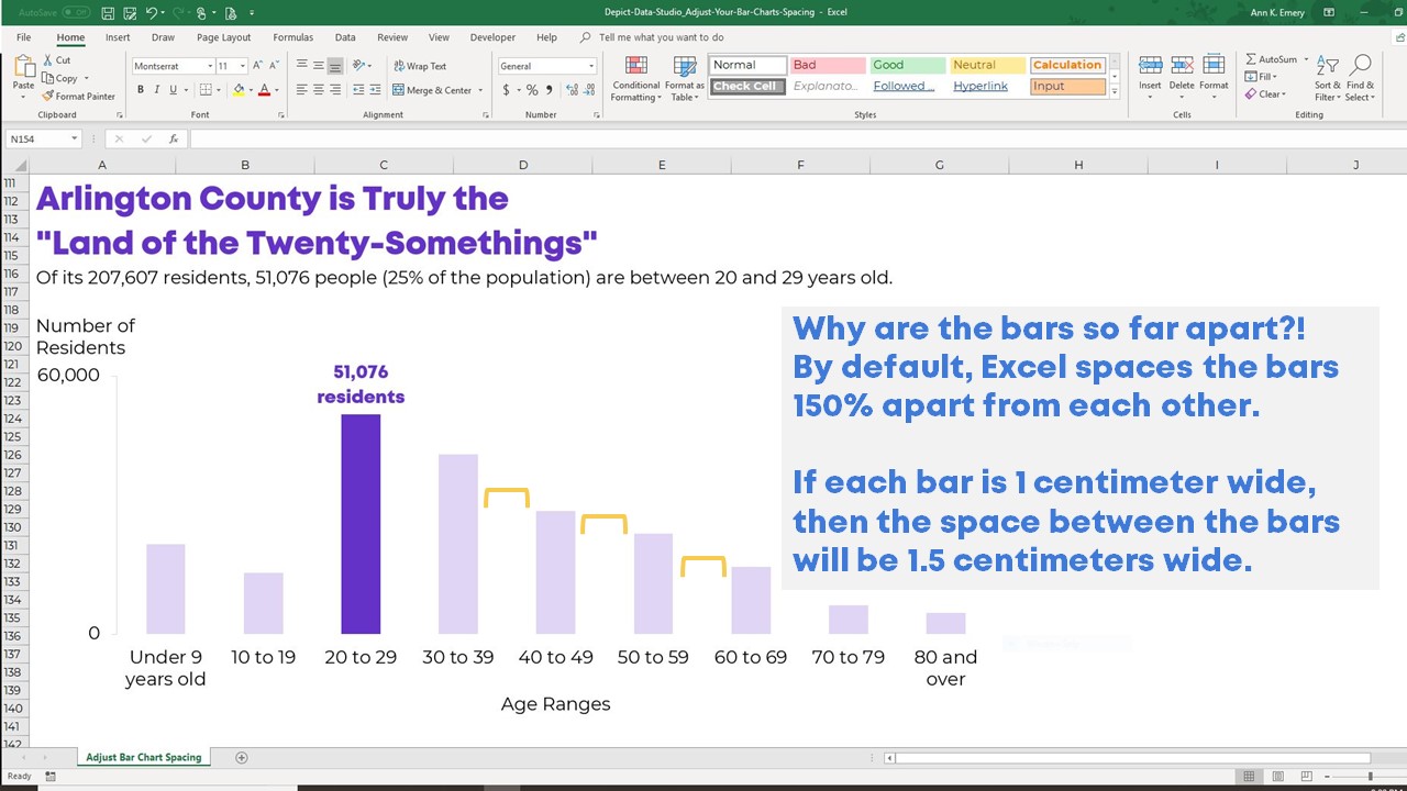
How to Adjust Your Bar Chart's Spacing in Microsoft Excel ...

› howto › 45677How to Create Progress Bars in Excel With Conditional Formatting Mar 11, 2011 · Progress Bars in Excel 2010 “Bar-type” conditional formatting has been around since Excel 2007. But Excel 2007 would only make bars with a gradient – the bar would get paler and paler towards the end, so even at 100% it wouldn’t really look like 100%. Excel 2010 addresses this by adding Solid Fill bars that maintain one color all ...

Placing labels on data points in a stacked bar chart in Excel ...

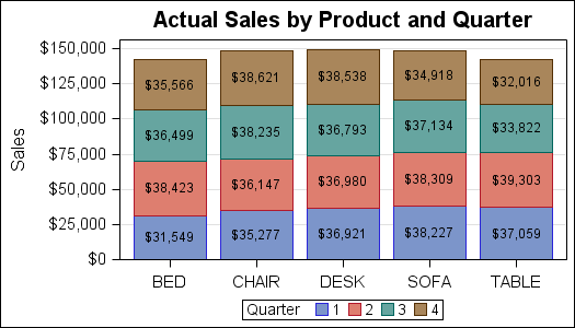
› color-chart-bars-by-valueHow to color chart bars based on their values - Get Digital Help May 11, 2021 · 3. How to color chart bars/columns based on multiple conditions? The image above demonstrates a chart that has bars/columns colored based on multiple conditions. It shows colored columns based on quarter, the color corresponds to the quarter number. 3.1 Prepare data. The image above shows the data, it is divided into four different columns.

Error bars in Excel: standard and custom

Bar Chart in Excel | Examples to Create 3 Types of Bar Charts Step 2: We will now select the whole table by clicking and dragging or placing the cursor anywhere in the table and pressing "CTRL+A" to choose the table completely. Step 3: Next, we will go to the "Insert" tab and move the cursor to the insert bar chart option.

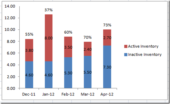
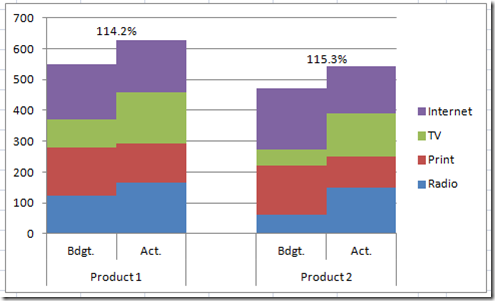
How-to Put Percentage Labels on Top of a Stacked Column Chart ...

› Make-a-Bar-Graph-in-ExcelHow to Make a Bar Graph in Excel: 9 Steps (with Pictures) May 02, 2022 · Open Microsoft Excel. It resembles a white "X" on a green background. A blank spreadsheet should open automatically, but you can go to File > New > Blank if you need to. If you want to create a graph from pre-existing data, instead double-click the Excel document that contains the data to open it and proceed to the next section.

How to Add Data Labels to an Excel 2010 Chart - dummies

How to add total labels to stacked column chart in Excel? - ExtendOffice Select and right click the new line chart and choose Add Data Labels > Add Data Labels from the right-clicking menu. See screenshot: And now each label has been added to corresponding data point of the Total data series. And the data labels stay at upper-right corners of each column. 5.

Custom Excel Chart Label Positions • My Online Training Hub

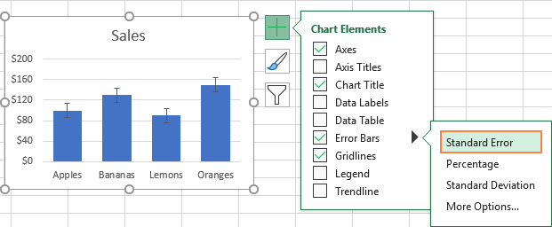
Error Bars in Excel (Examples) | How To Add Excel Error Bar? - EDUCBA To insert error bars, first, create a chart in Excel using any Bars or Columns charts, mainly from the Insert menu tab. Then click on the Plug button located at the right top corner of the chart and select Error Bars from there. To further customize the error bars choose More Options from the same menu list.

How to Make Your Excel Bar Chart Look Better – MBA Excel

Highlight Max & Min Values in an Excel Line Chart - Xelplus We will begin by creating a standard line chart in Excel using the below data set. Click anywhere in the data and select Insert (tab)-> Charts (group) -> Insert Line or Area Chart (button)-> Line with Markers (top row, second from right).. Using the newly created line chart, if we were to manually change the color of the highest value on the line, we would perform the following …

Add or remove data labels in a chart

8 Ways To Make Beautiful Financial Charts and Graphs in Excel 15.09.2021 · Aim to differentiate between a period and a series. Do this by minimizing white space in the blocks and between bars, and by making the bars wider. Tip #4: Remove background lines. As you can see below, there is a massive difference between the ‘before’ and ‘after’ Waterfall charts due to slight changes in design.

Align data labels in a graph so they are all along the same ...

How to Make a Bar Graph in Excel: 9 Steps (with Pictures) - wikiHow 02.05.2022 · Click on the element you want to adjust. For example, if you want to adjust the width of the bars, you would click on the bars. If that doesn't bring up options, try right clicking. Decreasing the gap width will make the bars appear to widen. If you have more than one set of data (i.e. the cost of two or more items over a given time span), you ...

How can I hide 0% value in data labels in an Excel Bar Chart ...

How to Add Total Values to Stacked Bar Chart in Excel Step 4: Add Total Values. Next, right click on the yellow line and click Add Data Labels. Next, double click on any of the labels. In the new panel that appears, check the button next to Above for the Label Position: Next, double click on the yellow line in the chart. In the new panel that appears, check the button next to No line:

Text Labels on a Vertical Column Chart in Excel - Peltier Tech

Bar Chart in Excel (Examples) | How to Create Bar Chart in Excel? - EDUCBA Step 9: To add Labels to the bar Right click on bar > Add Data Labels; click on it. Data Label is added to each bar. Similarly, you can choose different colors for each bar separately. I have chosen different colors, and my chart is looking like this. Example #2 There are multiple bar graphs available.

Change axis labels in a chart in Office

Find, label and highlight a certain data point in Excel ... - Ablebits 10.10.2018 · To let your users know which exactly data point is highlighted in your scatter chart, you can add a label to it. Here's how: Click on the highlighted data point to select it. Click the Chart Elements button. Select the Data Labels box and choose where to position the label. By default, Excel shows one numeric value for the label, y value in our ...

Add Percentage Labels to a 100% Stacked Bar chart in MS ...

Add or remove data labels in a chart - Microsoft Support Click Label Options and under Label Contains, pick the options you want. Use cell values as data labels You can use cell values as data labels for your chart. Right-click the data series or data label to display more data for, and then click Format Data Labels. Click Label Options and under Label Contains, select the Values From Cells checkbox.

Custom Y-Axis Labels in Excel - PolicyViz

How to Create a Milestone Chart in Excel - Excel Champs However, I have problem on last step. I am using your data sheet and unable to show different label name on this chart. If I change Placement Axis label range to activity name, the time/date label will also be changed to activity name at the same time. It’s hard to show different label name on two series line on last step. Reply

excel - How to show series-Legend label name in data labels ...

Labels | Product, Shipping & Address Labels | Staples® Label Shape. Label Type. All Filters. Sort by . Best Match. FEATURED PRODUCTS. Avery Easy Peel Laser/Inkjet Print-to-the-Edge Specialty Labels, 2" x 2", White, 300 Labels Per Pack (22806) Final price $21.49 $21.49. Add. Avery Kids No-Iron Fabric Labels, Assorted Sizes, White, 45/Pack (40700) Final price $7.99 $7.99 ...

How to add Axis Labels (X & Y) in Excel & Google Sheets ...

How to color chart bars based on their values - Get Digital Help 11.05.2021 · This article demonstrates two ways to color chart bars and chart columns based on their values. Excel has a built-in feature that allows you to color negative bars differently than positive values. You can even pick colors. You need to use a workaround if you want to color chart bars differently based on a condition.

How to Label Axes in Excel: 6 Steps (with Pictures) - wikiHow

How to Make a Bar Chart in Excel | Smartsheet Right-click the axis, click Format Axis, click Text Box, and enter an angle. You can also opt to only show some of the axis labels. Right-click the axis, click Format Axis, then click Scale, and enter a value in the Interval between labels box. A value of 2 will show every other label; 3 will show every third.

Add Labels ON Your Bars

How to Create and Print Barcode Labels From Excel and Word - enKo Products Select "All" then click "OK.". 16. The Word label template should now show the assigned text and barcodes. You may fix the label by realigning the text, resizing the barcode, setting image layout options to "Square," adding spaces or punctuations, etc. 17.

How to use data labels in a chart

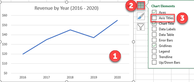
How to Make a Bar Chart in Microsoft Excel - How-To Geek To add axis labels to your bar chart, select your chart and click the green "Chart Elements" icon (the "+" icon). From the "Chart Elements" menu, enable the "Axis Titles" checkbox. Axis labels should appear for both the x axis (at the bottom) and the y axis (on the left). These will appear as text boxes.

Rule 24: Label your bars and axes — AddTwo

Creating & Labeling Small Multiple Bar Charts in Excel Step 1: Create gap or filler data. Create a gap or filler column of data for every category in your dataset. The real data and the filler data should add up to 100%. You can do this by entering the formula "=1-cell with the real data" in the gap column. For example, the formula for the gap column for Society for ages 65+ years would be ...

How to Add Axis Labels to a Chart in Excel | CustomGuide

How do I make excel label every bar in a bar chart? - Super User Insert->Pivot Chart Click Clustered Column Right-click on graph, select Format Axis set specify unit interval to 1 Excel now just labels every 2nd bar, even though it would easily fit (I have about 150 bars) with the given label font size. Even though I have selected 1, it has the same text density as if I set specify unit interval to 2.

Display Customized Data Labels on Charts & Graphs

How to Add Axis Labels in Excel Charts - Step-by-Step (2022) - Spreadsheeto Left-click the Excel chart. 2. Click the plus button in the upper right corner of the chart. 3. Click Axis Titles to put a checkmark in the axis title checkbox. This will display axis titles. 4. Click the added axis title text box to write your axis label. Or you can go to the 'Chart Design' tab, and click the 'Add Chart Element' button ...

Excel charts: add title, customize chart axis, legend and ...

How to add axis label to chart in Excel? - ExtendOffice Click to select the chart that you want to insert axis label. 2. Then click the Charts Elements button located the upper-right corner of the chart. In the expanded menu, check Axis Titles option, see screenshot: 3. And both the horizontal and vertical axis text boxes have been added to the chart, then click each of the axis text boxes and enter ...

How to Create a Bar Chart With Labels Inside Bars in Excel

HOW TO CREATE A BAR CHART WITH LABELS INSIDE BARS IN EXCEL - simplexCT 8. In the Format Data Labels pane, under Label Options selected, set the Label Position to Inside End. 9. Next, in the chart, select the Series 2 Data Labels and then set the Label Position to Inside Base. 10. Then, under Label Contains, check the Category Name option and uncheck the Value and Show Leader Lines options. 11.

How to add live total labels to graphs and charts in Excel ...

HOW TO CREATE A BAR CHART WITH LABELS ABOVE BAR IN EXCEL - simplexCT In the chart, right-click the Series "Dummy" Data Labels and then, on the short-cut menu, click Format Data Labels. 15. In the Format Data Labels pane, under Label Options selected, set the Label Position to Inside End. 16. Next, while the labels are still selected, click on Text Options, and then click on the Textbox icon. 17.

Aligning data point labels inside bars | How-To | Data ...

How to Add Total Data Labels to the Excel Stacked Bar Chart Step 5: Right click your new data labels and format them so that their label position is "Above"; also make the labels bold and increase the font size. Step 6: Right click the line, select "Format Data Series"; in the Line Color menu, select "No line" Step 7: Delete the "Total" data series label within the legend